Quick Start

Read data

Every pyextremes model starts with a pandas.Series (see pandas documentation) object, which contains timeseries of the data you want to analyze. This example is based on water level data for "The Battery" station located in New York.

Read data:

import pandas as pd

series = pd.read_csv(
    "battery_wl.csv",
    index_col=0,
    parse_dates=True,
).squeeze()

Tip

The battery_wl.csv file referenced above is used throughout many tutorials and examples for the pyextremes package. If you want to reproduce all steps shown here and get the same results, the file can be downloaded here.

---

Clean up data

In order for the analysis results to be meaningful, data needs to be pre-processed by the user. This may include removal of data gaps, detrending, interpolation, removal of outliers, etc. Let's clean up the data:

CodeWhen printed

series = (
    series
    .sort_index(ascending=True)
    .astype(float)
    .dropna()
    .loc[pd.to_datetime("1925"):]
)
series = series - (series.index.array - pd.to_datetime("1992")) / pd.to_timedelta("365.2425D") * 2.87e-3

print(series.head())

Date-Time (GMT)
1926-11-20 05:00:00   -0.411120
1926-11-20 06:00:00   -0.777120
1926-11-20 07:00:00   -1.051120
1926-11-20 08:00:00   -1.051121
1926-11-20 09:00:00   -0.808121
Name: Water Elevation [m NAVD88], dtype: float64

Note

See this tutorial for more information on why these specific operations were done.

---

Create model

The primary interface to the pyextremes library is provided via the EVA class. This class is responsible for all major tasks outlined above and is created using a simple command:

from pyextremes import EVA

model = EVA(series)

---

Extract extreme values

The first step of extreme value analysis is extraction of extreme values from the timeseries. This is done by using the get_extremes method of the EVA class.

In this example extremes will be extracted using the BM method and 1-year block_size, which give us annual maxima series.

CodeWhen printed

model.get_extremes(method="BM", block_size="365.2425D")

print(model.extremes.head())

Date-Time (GMT)
1927-02-20 16:00:00    1.670154
1927-12-05 10:00:00    1.432893
1929-04-16 19:00:00    1.409977
1930-08-23 01:00:00    1.202101
1931-03-08 17:00:00    1.529547
Name: Water Elevation [m NAVD88], dtype: float64

---

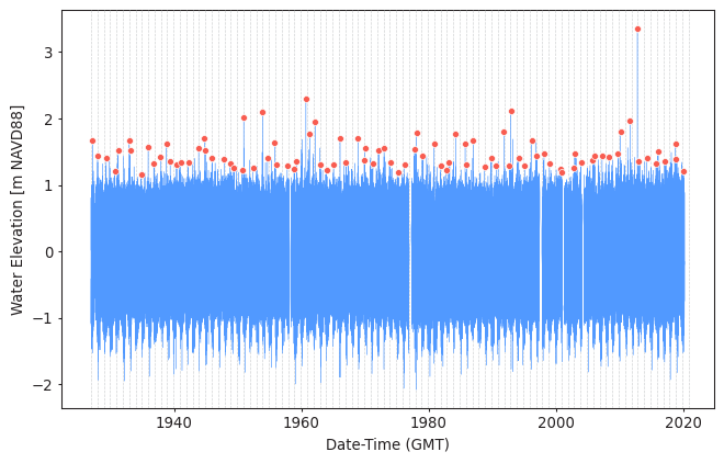
Visualize extreme events

model.plot_extremes()

---

Fit a model

The next step is selecting a model and fitting to the extracted extreme events. What this means practically is that we need to find model parameters (such as shape, location and scale for GEVD or GPD) that maximize or minimize some metric (likelihood) and give us the best fit possible. This is done by calling the fit_model method:

model.fit_model()

Info

By default, the fit_model method selects the best model applicable to extracted extremes using the Akaike Information Criterion (AIC).

---

Calculate return values

The final goal of most EVA's is estimation of return values. The simplest way to do this is by using the get_summary method:

summary = model.get_summary(
    return_period=[1, 2, 5, 10, 25, 50, 100, 250, 500, 1000],
    alpha=0.95,
    n_samples=1000,
)

Note

By default return period size is set to one year, which is defined as the mean year from the Gregorian calendar (365.2425 days). This means that a return period of 100 corresponds to a 100-year event.

A different return period size can be specified using the return_period_size argument. A value of 30D (30 days) would mean that a return period of 12 corresponds to approximately one year.

Print the results:

print(summary)

            return value  lower ci  upper ci
return period
1.0                0.802610 -0.270608  1.024385
2.0                1.409343  1.370929  1.452727
5.0                1.622565  1.540408  1.710116
10.0               1.803499  1.678816  1.955386
25.0               2.090267  1.851597  2.417670
50.0               2.354889  1.992022  2.906734
100.0              2.671313  2.145480  3.568418
250.0              3.188356  2.346609  4.856107
500.0              3.671580  2.517831  6.232830
1000.0             4.252220  2.702800  8.036243

---

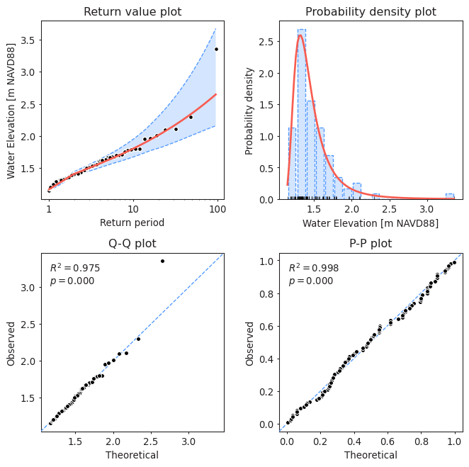
Investigate model

After model results are obtained, logical questions naturally arise - how good is the model, are the obtained results meaningful, and how confident can I be with the estimated return values. One way to do that is by visually inspecting the model:

model.plot_diagnostic(alpha=0.95)

---

Recap

Following this example you should be able to do the following:

• set up an EVA instance
• extract extreme events
• fit a model
• get results

For more in-depth tutorials on features of pyextremes see the User Guide.

---