Block Maxima
Block Maxima or Minima (BM) extreme values are extracted from time series by partitioning it into blocks (segments) of equal duration (e.g. 1 year) and locating maximum or minimum values within each block. Block maxima extreme values asymptotically follow the Generalized Extreme Value Distribution family, according to the Fisher–Tippett–Gnedenko theorem. This theorem demonstrates that the GEVD family is the only possible limit for the block maxima extreme values.
Extracting Extremes
As outlined in the Read First section of this documentation,
there are multiple ways the same thing can be achieved in pyextremes.
The BM extraction function can be accessed via:
pyextremes.extremes.block_maxima.get_extremes_block_maxima- the lowest levelpyextremes.get_extremes- general-purpose extreme value extraction functionpyextremes.EVA.get_extremes- helper-class (extreme values are not returned by this function, but instead are set on theEVAinstance in the.extremesattribute)
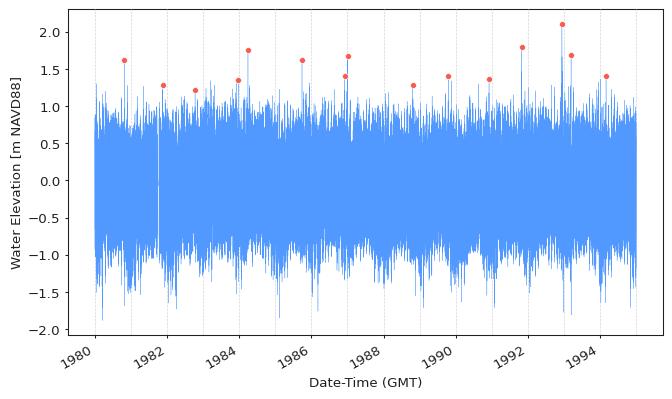
The simplest way to extract extreme values using BM method is to use the default
parameters of the get_extremes function:
from pyextremes import get_extremes
from pyextremes.plotting import plot_extremes

extremes = get_extremes(data, "BM")
plot_extremes(
    ts=data,
    extremes=extremes,
    extremes_method="BM",
    extremes_type="high",
    block_size="365.2425D",
)
from pyextremes import EVA

model = EVA(data=data)
model.get_extremes("BM")
model.plot_extremes()

Note
You can get the data variable referenced above by running the following code:
data = pd.read_csv(
    "battery_wl.csv",
    index_col=0,
    parse_dates=True,
).squeeze()
data = (
    data
    .sort_index(ascending=True)
    .astype(float)
    .dropna()
    .loc[pd.to_datetime("1980"):pd.to_datetime("1995")]
)
data = (
  data - (data.index.array - pd.to_datetime("1992"))
) / pd.to_timedelta("365.2425D") * 2.87e-3
"battery_wl.csv"
can be downloaded here.
All figures shown in this tutorial section were generated using this jupyter notebook.
The get_extremes function uses the following parameters:
- ts - time series (
pandas.Series) from which the extreme values are extracted - method - extreme value extraction method:
"BM"for Block Maxima and"POT"for Peaks Over Threshold. - extremes_type - extreme value type:
"high"for maxima (default) and"low"for minima
The following paramters are used only when method="BM":
- block_size - block size, by default
"365.2425D". Internally is converted using thepandas.to_timedeltafunction. - errors - specifies what to do when a block is empty (has no values).
"raise"(default) raises error,"ignore"skips such blocks (not recommended), and"coerce"sets values for such blocks as average of extreme values in other blocks. - min_last_block - minimum data availability ratio (0 to 1)
in the last block. If the last block is shorter than this ration
(e.g. 0.25 corresponds to 3 months for a block size of 1 year) then it is not used
to get extreme values. This argument is useful to avoid situations when the last
block is very small. By default this is
None, which means that last block is always used.
If we specify all of these parameters then the function would look as:
get_extremes(
    ts=data,
    method="BM",
    extremes_type="high",
    block_size="365.2425D",
    errors="raise",
    min_last_block=None,
)
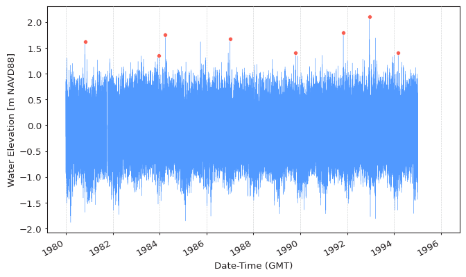
Selecting Block Size
Like with most choices in statistics, selection of block size involves making a trade-off between bias and variance: blocks that are too small mean that approximation by the limit model (GEVD) is likely to be poor, leading to bias in estimation and extrapolation; large blocks generate few block maxima/minima, leading to large estimation variance. Pragmatic considerations often lead to the adoption of blocks of length one year. (Coles, 2004)
An important thing to consider is also the physical nature of investigated signal. Many meteorological events (e.g. snowfall, rain, waves) are seasonal and, therefore, selection of block sizes smaller than 1-year would result in significant bias due to blocks no longer being equivalent (e.g. summer blocks are nearly guaranteed to have no snow).
We can specify different block size using the block_size argument. Using the same
data as above but with a block size of 2 years we get:
extremes = get_extremes(
    ts=data,
    method="BM",
    block_size=pd.to_timedelta("365.2425D") * 2,
)
plot_extremes(
    ts=data,
    extremes=extremes,
    extremes_method="BM",
    extremes_type="high",
    block_size=pd.to_timedelta("365.2425D") * 2,
)
model = EVA(data=data)
model.get_extremes("BM", block_size=pd.to_timedelta("365.2425D") * 2)
model.plot_extremes()
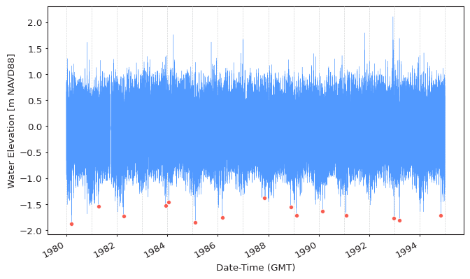
Block Minima
Block minima is fully equivalent to block maxima in the way it is extracted.
Block minima can be extracted by setting the extremes_type argument
to "low":
extremes = get_extremes(
    ts=data,
    method="BM",
    extremes_type="low",
)
plot_extremes(
    ts=data,
    extremes=extremes,
    extremes_method="BM",
    extremes_type="high",
    block_size="365.2425D",
)
model = EVA(data=data)
model.get_extremes("BM", extremes_type="low")
model.plot_extremes()
Tip
The pyextremes.EVA class works identically for both maxima and minima series and
properly reflects (rotates) the data to fit statistical distributions.
This is true as long as the extremes_type argument is correctly specified.
Warning
When analyzing block minima be mindful of your data being censored. An example of this would be water level time series - water levels cannot go below the seabed and will, therefore, be censored by the seabed elevation. Such series would no longer follow the GEVD and any results of such analysis would be unreliable.