Estimating Return Periods
This section demonstrates how empirical probabilities (return periods) can be obtained for extreme values extracted using methods described in earlier sections.
What is Return Period
Return period indicates duration of time (typically years) which corresponds to a
probability that a given value (e.g. wind speed) would be exceeded at least once within
a year. This probability is called probability of exceedance and is related to return
periods as 1/p where p is return period.
Coles (2001, p.49)
In common terminology, \(z_{p}\) is the return level associated with the return period \(1/p\), since to a reasonable degree of accuracy, the level \(z_{p}\) is expected to be exceeded on average once every \(1/p\) years. More precisely, \(z_{p}\) is exceeded by the annual maximum in any particular year with probability \(p\).
Return periods are often incorrectly interpreted in the professional communities as "100-year event is an event which happens only once in 100 years", which may lead to inaccurate assessment of risks. A more holistic way of looking at this is to consider a time period within which a risk is evaluated. For example, a 100-year event with probability of exceedance in any given year of 1% would have a probability of ~39.5% to be exceeded at least once within 50 years - this is calculated using this formula:
Where \(n\) is number of return period blocks within a time period (50 for 50 years with retun period block of size 1 year) and \(p\) is 1% (100-year event).
Empirical Return Periods
Empirical return periods are assigned to observed extreme values using an empirical rule
where extreme values are ordered and ranked from the most extreme (1) to the
least extreme (n), then exceedance probabilities are calculated
(see the following sub-section), and return periods are calculated as multiples of
a given return_period_size (typically 1 year).
Probability of Exceedance
Extreme events extracted using BM or POT methods are assigned exceedance probabilities using the following formula:
where:
- r - rank of extreme value (1 to n). In
pyextremesrank is calculated usingscipy.stats.rankdatawithmethod="average", which means that extreme events of the same magnitude are assigned average of ranks these values would be assigned otherwise if ranked sequentially. For example, array of[1, 2, 3, 3, 4]would have ranks of[5, 4, 2.5, 2.5, 1]. - n - number of extreme values.
- \(\alpha\) and \(\beta\) - empricial plotting position parameters (see further below).
In this context \(P\) corresponds to a probability of exceedance of a value with rank r in a any given time period with duration \(t/n\) where \(t\) is total duration of series from which the extreme values were drawn and \(n\) is number of extreme events. If we measure time in years and we use Block Maxima with block size of 1 year, then the formula \(t/n\) becomes 1 by definition and the return period in years can be calculated as \(1/P\). For general rule read this tutorial section further.
Plotting Positions
Plotting positions are sets of empirical coefficients defining how extreme values are assigned probabilities, which are subsequently used to plot extreme values on the probability plots.
Warning
Plotting positions have nothing to do with modeling extreme event statistics in modern EVA. Historically, in time before computers became widespread, EVA was performed by plotting extreme events on probability paper (with axes scaled logarithmically and according to a specific plotting position) with the idea that a return value curve for a given model (e.g. GEVD) would be a straight line drawn through these points using a pen and a ruler.
Modern EVA fits models to data by maximimizng likelihood function via methods such as MLE or MCMC (read more in other sections). This is only feasible due to the use of computers and would be prohibitively expensive to do manually. Plotting positions are presently used only to show extreme values on return value plots and to perform some goodness-of-fit tests (e.g. P-P or Q-Q plots).
TL;DR: plotting positions are NOT used to fit models.
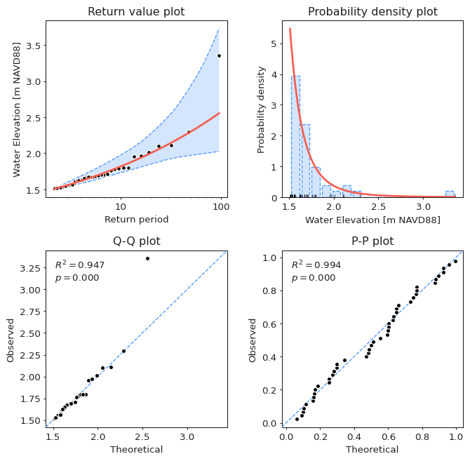
An example of plotting positions used in pyextremes is the diagnostic plot where
observed extreme values (black dots) are superimposed against the theoretical
estimates (by fitting a distribution) as seen in the return value, Q-Q, and P-P plots.
Return Period
Return periods are calculated from the exceedance probabilities using the following formula:
where:
- R - return period as multiple of
return_period_size(by default 1 year). - P - exceedance probability calculated earlier.
- \(\lambda\) - rate of extreme events (average number of extreme events per
return_period_size). Calculated as:- \(\lambda\) =
return_period_size/block_sizefor Block Maxima - \(\lambda = \frac{n}{t / return\_period\_size}\) for Peaks Over Threshold, where \(n\) is number of extreme events and \(t\) is total duration of series from which the extreme values were drawn
- \(\lambda\) =
The resulting return period R is, therefore, a real number representing a multiple
of return_period_size.
Example
We have 2 years of data and, using block_size of 30 days (~1 month), we extract
24 extreme events using the Block Maxima method. We then rank the values from 1
to 24 as outlined above and, using the Weibull plotting position
(\(\alpha=0\) and \(\beta=0\)), for the most extreme value (rank 1)
we get exceedance probability \(P\) of 1/25 or 0.04.
Let's say we would like to get return period of the most extreme value (rank 1)
in years (return_period_size of 1 year). First, we calculate extreme value rate
\(\lambda\) as return_period_size / block_size, which gives us 12 (approximately
since we used 30 days for block_size). Now we can use the return period formula
above directly as \(R = 1 / 0.04 / 12 = 2.08\) years.
Estimating Return Periods
pyextremes estimates empirical return periods for many plotting functions and
goodness-of-fit tests behind the scenes using the Weibull plotting position.
Return periods can be calculated using the get_return_periods function (shown only
for Block Maxima; Peaks Over Threshold works identically with the only difference
being the block_size argument):
from pyextremes import get_extremes, get_return_periods

extremes = get_extremes(
    ts=data,
    method="BM",
    block_size="365.2425D",
)
return_periods = get_return_periods(
    ts=data,
    extremes=extremes,
    extremes_method="BM",
    extremes_type="high",
    block_size="365.2425D",
    return_period_size="365.2425D",
    plotting_position="weibull",
)
return_periods.sort_values("return period", ascending=False).head()
| Date-Time (GMT) | Water Elevation [m NAVD88] | exceedance probability | return period |
|---|---|---|---|
| 2012-10-30 01:00:00 | 3.357218 | 0.010526 | 95.000000 |
| 1960-09-12 18:00:00 | 2.295832 | 0.021053 | 47.500000 |
| 1992-12-11 14:00:00 | 2.108284 | 0.031579 | 31.666667 |
| 1953-11-07 12:00:00 | 2.101487 | 0.042105 | 23.750000 |
| 1950-11-25 14:00:00 | 2.012957 | 0.052632 | 19.000000 |
from pyextremes import get_extremes, get_return_periods

extremes = get_extremes(
    ts=data,
    method="BM",
    block_size="365.2425D",
)
return_periods = get_return_periods(
    ts=data,
    extremes=extremes,
    extremes_method="BM",
    extremes_type="high",
    block_size="365.2425D",
    return_period_size="365.2425D",
    plotting_position="median",
)
return_periods.sort_values("return period", ascending=False).head()
| Date-Time (GMT) | Water Elevation [m NAVD88] | exceedance probability | return period |
|---|---|---|---|
| 2012-10-30 01:00:00 | 3.357218 | 0.007233 | 138.263736 |
| 1960-09-12 18:00:00 | 2.295832 | 0.017830 | 56.086181 |
| 1992-12-11 14:00:00 | 2.108284 | 0.028427 | 35.178006 |
| 1953-11-07 12:00:00 | 2.101487 | 0.039024 | 25.625255 |
| 1950-11-25 14:00:00 | 2.012957 | 0.049621 | 20.152696 |
from pyextremes import get_extremes, get_return_periods

extremes = get_extremes(
    ts=data,
    method="BM",
    block_size="365.2425D",
)
return_periods = get_return_periods(
    ts=data,
    extremes=extremes,
    extremes_method="BM",
    extremes_type="high",
    block_size="365.2425D",
    return_period_size="365.2425D",
    plotting_position="cunnane",
)
return_periods.sort_values("return period", ascending=False).head()
| Date-Time (GMT) | Water Elevation [m NAVD88] | exceedance probability | return period |
|---|---|---|---|
| 2012-10-30 01:00:00 | 3.357218 | 0.006369 | 157.000000 |
| 1960-09-12 18:00:00 | 2.295832 | 0.016985 | 58.875000 |
| 1992-12-11 14:00:00 | 2.108284 | 0.027601 | 36.230769 |
| 1953-11-07 12:00:00 | 2.101487 | 0.038217 | 26.166667 |
| 1950-11-25 14:00:00 | 2.012957 | 0.048832 | 20.478261 |
from pyextremes import get_extremes, get_return_periods

extremes = get_extremes(
    ts=data,
    method="BM",
    block_size="365.2425D",
)
return_periods = get_return_periods(
    ts=data,
    extremes=extremes,
    extremes_method="BM",
    extremes_type="high",
    block_size="365.2425D",
    return_period_size="365.2425D",
    plotting_position="gringorten",
)
return_periods.sort_values("return period", ascending=False).head()
| Date-Time (GMT) | Water Elevation [m NAVD88] | exceedance probability | return period |
|---|---|---|---|
| 2012-10-30 01:00:00 | 3.357218 | 0.005950 | 168.071429 |
| 1960-09-12 18:00:00 | 2.295832 | 0.016575 | 60.333333 |
| 1992-12-11 14:00:00 | 2.108284 | 0.027199 | 36.765625 |
| 1953-11-07 12:00:00 | 2.101487 | 0.037824 | 26.438202 |
| 1950-11-25 14:00:00 | 2.012957 | 0.048449 | 20.640351 |
The get_return_periods function uses the following parameters:
- ts - time series (
pandas.Series) from which the extreme values are extracted - extremes - time series of extreme values.
- extremes_method - extreme value extraction method, must be
"BM"or"POT". - extremes_type - extreme value type:
"high"for above threshold (default) and"low"for below threshold. - return_period_size - size of return period. Same as the
rargument. By default this is 1 year. - plotting_position : plotting position name, case-insensitive. Supported plotting positions: ecdf, hazen, weibull (default), tukey, blom, median, cunnane, gringorten, beard.
The following paramters are used only when extremes_method="BM":
- block_size - block size, by default
"365.2425D". Internally is converted using thepandas.to_timedeltafunction. If not provided, then it is calculated as median distance between extreme values.
Note
You can get the data variable referenced above by running the following code:
data = pd.read_csv(
    "battery_wl.csv",
    index_col=0,
    parse_dates=True,
).squeeze()
data = (
    data
    .sort_index(ascending=True)
    .astype(float)
    .dropna()
    .loc[pd.to_datetime("1925"):]
)
data = (
  data - (data.index.array - pd.to_datetime("1992"))
) / pd.to_timedelta("365.2425D") * 2.87e-3
"battery_wl.csv"
can be downloaded here.
All figures shown in this tutorial section were generated using this jupyter notebook.