Threshold Selection

Selection of the threshold value is a very important step because it has the strongest effect on the results of EVA. The core idea of threshold selection is the same as when selecting block size in the Block Maxima approach - it is a trade-off between bias and variance. Larger threshold values produce few extreme values and lead to large variance in result (confidence bounds), while smaller threshold values generate a sample which poorly approximates the GPD model. The opposite is true when performing EVA for extreme low values (extremes_type="low").

The key goal of threshold selection can, therefore, be formulated as follows:

Goal of threshold selection

Select the smallest threshold value among those which produce extreme values following the limit exceedance model (Generalized Pareto Distribution family).

Warning

Threshold selection is probably the hardest part of Extreme Value Analysis when analyzing extreme values obtained using the Peaks Over Threshold method. It involves a great deal of subjective judgement and should be performed in conjunction with other methods, such as Block Maxima + GEVD, to gain more confidence in the validty of obtained results.

Mean Residual Life¶

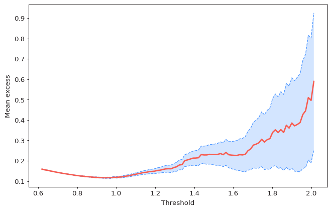
Mean residual life plot plots average excess value over given threshold for a series of thresholds. The idea is that the mean residual life plot should be approximately linear above a threshold for which the Generalized Pareto Distribution model is valid.

from pyextremes import plot_mean_residual_life

plot_mean_residual_life(data)

Note

You can get the data variable referenced above by running the following code:

data = pd.read_csv(
    "battery_wl.csv",
    index_col=0,
    parse_dates=True,
).squeeze()
data = (
    data
    .sort_index(ascending=True)
    .astype(float)
    .dropna()
    .loc[pd.to_datetime("1925"):]
)
data = (
  data - (data.index.array - pd.to_datetime("1992"))
) / pd.to_timedelta("365.2425D") * 2.87e-3

"battery_wl.csv" can be downloaded here.

All figures shown in this tutorial section were generated using this jupyter notebook.

As seen in the figure above, exceedance values are approximately linear between threshold values of 1.2 and 1.8. This provides a range of threshold values which can be further investigated using other methods.

The plot_mean_residual_life function uses the following parameters:

ts - time series (pandas.Series) from which the extreme values are extracted
thresholds - array of threshold for which the plot is displayed. By default 100 equally-spaced thresholds between 90th (10th if extremes_type="high") percentile and 10th largest (smallest if extremes_type="low") value in the series.
extremes_type - extreme value type: "high" for above threshold (default) and "low" for below threshold.
alpha - confidence interval width in the range (0, 1), by default it is 0.95. If None, then confidence interval is not shown.
ax - matplotlib Axes object. If provided, then the plot is drawn on this axes. If None (default), new figure and axes are created
figsize - figure size in inches in format (width, height). By default it is (8, 5).

Note

In author's (subjective) opinion this is the least useful technique among those listed in this section because mean residual life plots are very hard to interpret.

Parameter Stability¶

Parameter stability plot shows how shape and modified scale parameters of the Generalized Pareto Distribution change over a range of threshold values. The idea is that these parameters should be stable (vary by small amount) within a range of valid thresholds.

from pyextremes import plot_parameter_stability

plot_parameter_stability(data)

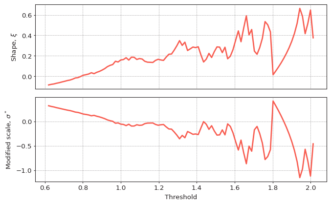
As seen in the figure above, these parameters appear to stabilize around threshold value of 1.2 with subsequent values having higher variance due to smaller number of exceedances.

The plot_parameter_stability function uses the following parameters:

ts - time series (pandas.Series) from which the extreme values are extracted
thresholds - array of threshold for which the plot is displayed. By default 100 equally-spaced thresholds between 90th (10th if extremes_type="high") percentile and 10th largest (smallest if extremes_type="low") value in the series.
r - minimum time distance (window duration) between adjacent clusters. Used to decluster exceedances by locating clusters where all exceedances are separated by distances no more than r and then locating maximum or minimum (depends on extremes_type) values within each cluster. By default r="24H" (24 hours).
extremes_type - extreme value type: "high" for above threshold (default) and "low" for below threshold.
alpha - confidence interval width in the range (0, 1), by default it is 0.95. If None, then confidence interval is not shown.
n_samples - number of bootstrap samples used to estimate confidence interval bounds (default=100). Ignored if alpha is None.
axes - tuple with matplotlib Axes (ax_shape, ax_scale) for shape and scale values. If None (default), new figure and axes are created.
figsize - figure size in inches in format (width, height). By default it is (8, 5).
progress - if True, shows tqdm progress bar. By default False. Requires tqdm package.

Return Value Stability¶

An extension of the previous technique is to investigate stability of a target return value with a pre-defined return period over a range of thresholds. This technique provides a more intuitive metric of model stability. Let's plot it for the range of thresholds identified earlier:

from pyextremes import plot_return_value_stability

plot_return_value_stability(
    data,
    return_period=100,
    thresholds=np.linspace(1.2, 1.8, 20),
    alpha=0.95,
)

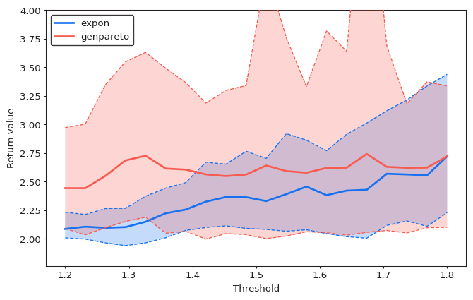
As seen in the figure above, the model is very stable for threshold values above 1.4.

The plot_return_value_stability function uses the following parameters:

ts - time series (pandas.Series) from which the extreme values are extracted
return_period - return period given as a multiple of return_period_size.
return_period_size - size of return period. Same as the r argument. By default this is 1 year.
thresholds - array of threshold for which the plot is displayed. By default 100 equally-spaced thresholds between 90th (10th if extremes_type="high") percentile and 10th largest (smallest if extremes_type="low") value in the series.
r - minimum time distance (window duration) between adjacent clusters. Used to decluster exceedances by locating clusters where all exceedances are separated by distances no more than r and then locating maximum or minimum (depends on extremes_type) values within each cluster. By default r="24H" (24 hours).
extremes_type - extreme value type: "high" for above threshold (default) and "low" for below threshold.
distributions - list of distributions for which the plot is produced. By default these are "genpareto" and "expon". A distribution must be either a name of distribution from scipy.stats or a subclass of scipy.stats.rv_continuous. See scipy.stats documentation
alpha - confidence interval width in the range (0, 1), by default it is 0.95. If None, then confidence interval is not shown.
n_samples - number of bootstrap samples used to estimate confidence interval bounds (default=100). Ignored if alpha is None.
ax - matplotlib Axes object. If provided, then the plot is drawn on this axes. If None (default), new figure and axes are created
figsize - figure size in inches in format (width, height). By default it is (8, 5).
progress - if True, shows tqdm progress bar. By default False. Requires tqdm package.

Warning

This is the most dangerous threshold selection teqchnique presented in this section. It can be abused by selecting a threshold value which gives a desired result. Results of such analysis would be biased and invalid. Analyst should honestly present results of their analysis and high variance in answer should be considered a valuable result as well - it indicates that available data cann be used to obtain reliable results and that there is high uncertainty in the analyzed process.

Putting it all Together¶

pyextremes provides a convenience function to put all of the above together. It also adds an additional plot - AIC curve indicating relative model performance. The AIC curve should not be used as a threshold selection tool because it will always have the same logarithmic shape. Instead, it should guide the user as to which model (e.g. GEVD or Exponential) should be preferred for a given threshold.

from pyextremes import plot_threshold_stability

plot_threshold_stability(
    data,
    return_period=100,
    thresholds=np.linspace(1.2, 1.8, 20),
)

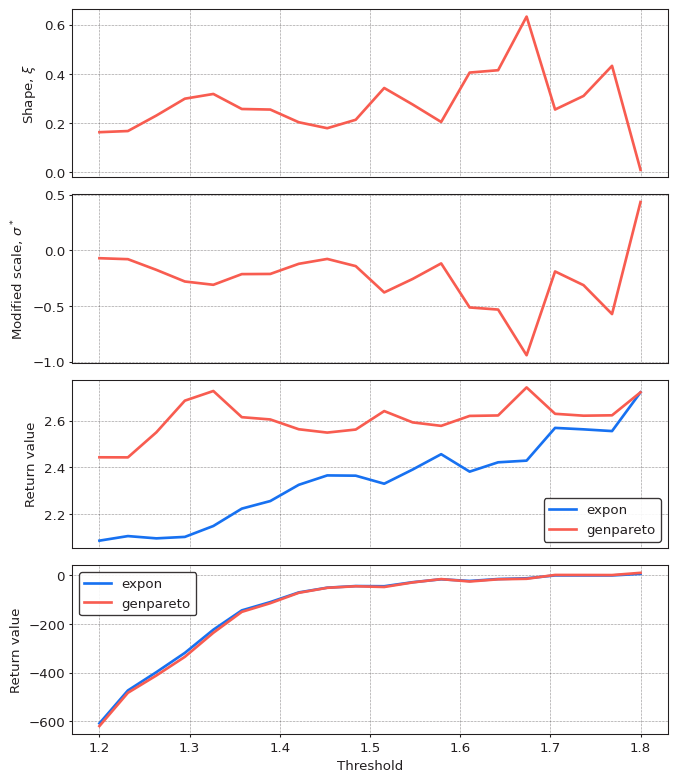
Based on the figures shown earlier, one may conclude that the valid threshold may lie between 1.4 and 1.6. A decision was made to select threshold value of 1.5.

The plot_threshold_stability function uses the following parameters:

ts - time series (pandas.Series) from which the extreme values are extracted
return_period - return period given as a multiple of return_period_size.
return_period_size - size of return period. Same as the r argument. By default this is 1 year.
thresholds - array of threshold for which the plot is displayed. By default 100 equally-spaced thresholds between 90th (10th if extremes_type="high") percentile and 10th largest (smallest if extremes_type="low") value in the series.
r - minimum time distance (window duration) between adjacent clusters. Used to decluster exceedances by locating clusters where all exceedances are separated by distances no more than r and then locating maximum or minimum (depends on extremes_type) values within each cluster. By default r="24H" (24 hours).
extremes_type - extreme value type: "high" for above threshold (default) and "low" for below threshold.
distributions - list of distributions for which the plot is produced. By default these are "genpareto" and "expon". A distribution must be either a name of distribution from scipy.stats or a subclass of scipy.stats.rv_continuous. See scipy.stats documentation
alpha - confidence interval width in the range (0, 1), by default it is 0.95. If None, then confidence interval is not shown.
n_samples - number of bootstrap samples used to estimate confidence interval bounds (default=100). Ignored if alpha is None.
ax - matplotlib Axes object. If provided, then the plot is drawn on this axes. If None (default), new figure and axes are created
figsize - figure size in inches in format (width, height). By default it is (8, 5).
progress - if True, shows tqdm progress bar. By default False. Requires tqdm package.

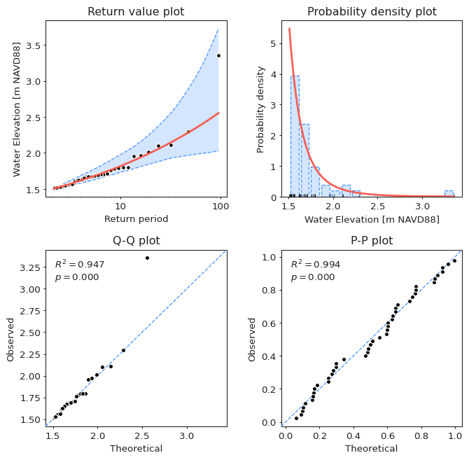
Results of selecting the threshold value 1.5 are shown below: