Extreme Low Values

Extreme value theory and the distributions used in EVA (GEVD, GPD, and their degenerate cases) describe extreme high values: the right tail of a distribution. Extreme low values, such as block minima or peaks below a threshold (see Block Maxima and Peaks Over Threshold), are analyzed by transforming them into extreme high values, fitting a model, and transforming the results back.

Transformation¶

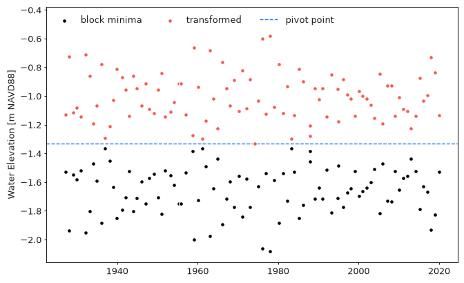
The transformation reflects the extreme values around a pivot point, which is the largest of the extreme low values:

\[x' = 2 x_{pivot} - x\]

After the transformation the most extreme (lowest) values become the largest ones, while the values stay in the same units and in the same range as the original data. Applying the same formula again returns the original values. The transformation is implemented in the ExtremesTransformer class:

from pyextremes.extremes import ExtremesTransformer

transformer = ExtremesTransformer(extremes=extremes, extremes_type="low")
transformer.pivot_point  # -1.331
transformer.transformed_extremes  # reflected extremes
transformer.transform(-2.0)  # transform any value in either direction

Note

You can get the data and extremes variables referenced in this section by running the following code:

import pandas as pd
from pyextremes import get_extremes

data = pd.read_csv(
    "battery_wl.csv",
    index_col=0,
    parse_dates=True,
).squeeze()
data = (
    data
    .sort_index(ascending=True)
    .astype(float)
    .dropna()
    .loc[pd.to_datetime("1925"):]
)
data = (
    data
    - (data.index.array - pd.to_datetime("1992"))
    / pd.to_timedelta("365.2425D")
    * 2.87e-3
)

extremes = get_extremes(data, "BM", extremes_type="low", block_size="365.2425D")

"battery_wl.csv" can be downloaded here.

For extreme high values (extremes_type="high") no transformation is performed: the pivot point is None and transform returns values unchanged.

Using EVA¶

EVA applies the transformation automatically whenever the extreme values were extracted with extremes_type="low":

models are fitted to the transformed extremes
the location parameter of genpareto and expon distributions is fixed at the transformed threshold (see Distributions)
return values, confidence intervals, and plots are transformed back, so all results are in the original units and direction

Block MinimaPeaks Below Threshold

from pyextremes import EVA

model = EVA(data=data)
model.get_extremes("BM", extremes_type="low", block_size="365.2425D")
model.fit_model()
summary = model.get_summary(
    return_period=[2, 10, 100],
    alpha=0.95,
    n_samples=1000,
)
print(summary)

               return value  lower ci  upper ci
return period
2.0               -1.642462 -1.607109 -1.679627
10.0              -1.871511 -1.820393 -1.917212
100.0             -2.070594 -1.971140 -2.163691

from pyextremes import EVA

model = EVA(data=data)
model.get_extremes("POT", extremes_type="low", threshold=-1.6, r="24h")
model.fit_model()
summary = model.get_summary(
    return_period=[5, 10, 100],
    alpha=0.95,
    n_samples=1000,
)
print(summary)

               return value  lower ci  upper ci
return period
5.0               -1.808288 -1.767934 -1.845680
10.0              -1.881013 -1.831928 -1.921228
100.0             -2.057187 -1.960945 -2.146891

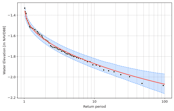
The 100-year low water level is about -2.06 m to -2.07 m for both extraction methods. Longer return periods correspond to lower water levels (shown for the block minima model):

import numpy as np

model.plot_return_values(
    return_period=np.logspace(0.01, 2, 100),
    alpha=0.95,
    n_samples=1000,
)

Confidence interval columns

For extreme low values, lower ci and upper ci refer to the bounds of the interval in the transformed space. After transforming back, lower ci is the less extreme bound (the higher water level) and upper ci is the more extreme bound (the lower water level), so numerically lower ci is larger than upper ci, as seen in the tables above.

Censored data

Extreme low values are often censored by a physical limit (e.g. water levels can't drop below the seabed). Censored extreme values don't follow the extreme value distributions and their analysis would be unreliable.

Standalone Usage¶

The standalone get_model function fits the distribution to the extreme values exactly as provided. To analyze extreme low values without EVA, transform them first and transform the return values back:

CodeOutput

from pyextremes import get_extremes, get_model
from pyextremes.extremes import ExtremesTransformer

extremes = get_extremes(data, "BM", extremes_type="low", block_size="365.2425D")
transformer = ExtremesTransformer(extremes=extremes, extremes_type="low")
model = get_model(
    model="MLE",
    extremes=transformer.transformed_extremes,
    distribution="genextreme",
)
return_value, _, _ = model.get_return_value(exceedance_probability=0.01)
print(transformer.transform(return_value))

-2.070593655775087

When fitting genpareto or expon to peaks below a threshold this way, fix the location parameter at the transformed threshold, i.e. distribution_kwargs={"floc": transformer.transform(threshold)}.