Markov Chain Monte Carlo

Markov Chain Monte Carlo (MCMC) is a Bayesian approach to fitting a model. Instead of finding a single best set of distribution parameters \(\theta\), it draws samples from the posterior distribution of the parameters given the observed extreme values \(x\):

where \(L(x \mid \theta)\) is the likelihood (same as in MLE) and \(p(\theta)\) is the prior distribution of the parameters. pyextremes uses a flat (uninformative) prior, which means that the posterior is proportional to the likelihood and the results are driven by the data alone.

The resulting samples describe the full joint uncertainty of all distribution parameters, which is then propagated directly to return values. This makes MCMC a good way to verify confidence intervals obtained using MLE, especially for small samples, where the bootstrap may be unreliable.

pyextremes implements MCMC in the Emcee model, which uses the affine-invariant ensemble sampler from the emcee package by Dan Foreman-Mackey et al.

Fitting the Model¶

from pyextremes import get_extremes, get_model

extremes = get_extremes(data, "BM", block_size="365.2425D")
model = get_model(
    model="Emcee",
    extremes=extremes,
    distribution="genextreme",
    n_walkers=100,
    n_samples=1000,
)

from pyextremes import EVA

model = EVA(data=data)
model.get_extremes("BM", block_size="365.2425D")
model.fit_model(model="Emcee", n_walkers=100, n_samples=1000)

import pandas as pd

data = pd.read_csv(
    "battery_wl.csv",
    index_col=0,
    parse_dates=True,
).squeeze()
data = (
    data
    .sort_index(ascending=True)
    .astype(float)
    .dropna()
    .loc[pd.to_datetime("1925"):]
)
data = (
    data
    - (data.index.array - pd.to_datetime("1992"))
    / pd.to_timedelta("365.2425D")
    * 2.87e-3
)

The Emcee model takes the following additional arguments:

• n_walkers - number of walkers in the ensemble, by default 100. Each walker is an independent chain exploring the parameter space. Walkers start near the MLE estimate of the distribution parameters.
• n_samples - number of steps each walker takes, by default 500. The total number of posterior samples is n_walkers * n_samples.
• progress - if True, shows a progress bar while sampling. By default False. A string (e.g. "notebook") selects a specific tqdm progress bar. Requires the tqdm package.
• pool - a pool object with a map method (e.g. multiprocessing.Pool) used to evaluate walkers in parallel. By default None (no parallelization).

The fitted model has the following properties:

print(model.model)
print(model.model.trace.shape)

                   Emcee model
-------------------------------------------------
free parameters: c=-0.264, loc=1.352, scale=0.145
fixed parameters: all parameters are free
AIC: -29.779
loglikelihood: 18.023
number of walkers: 100
number of samples: 1000
return value cache size: 0
-------------------------------------------------
(100, 1000, 3)

The trace attribute holds all posterior samples as an array with shape (n_walkers, n_samples, n_free_parameters). The fitted parameters (fit_parameters) are the maximum a posteriori (MAP) estimate - the mode of the posterior distribution, estimated using a Gaussian kernel density estimate over all samples in the trace. With a flat prior the MAP estimate is equivalent to the MLE estimate, which is why the parameters above are nearly identical to those obtained using MLE (c=-0.266, loc=1.353, scale=0.146).

import multiprocessing

if __name__ == "__main__":
    ...
    with multiprocessing.Pool() as pool:
        model.fit_model(model="Emcee", n_samples=1000, pool=pool)

Burn-in¶

Walkers need some number of steps to move away from their starting positions and converge to the posterior distribution. Samples taken during this burn-in period are not representative of the posterior and should be discarded. The trace plot shows how the walkers explore the parameter space and helps choose the burn-in value:

model.plot_trace()

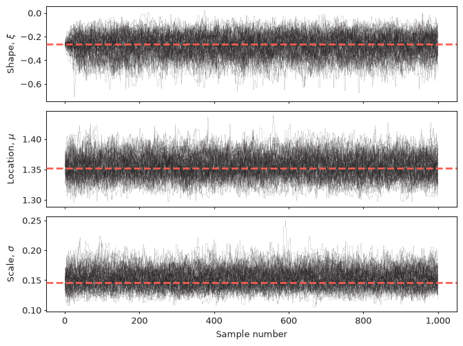
Each black line is a walker and the red dashed line is the MAP estimate. Walkers start in a tight cluster (around the MLE estimate) and spread out over the first few dozen steps, after which the chains look stationary (i.e. they fluctuate around a stable mean with a stable spread). Here, discarding the first 200 samples is a conservative choice.

The burn-in value is passed using the burn_in argument (by default 0, meaning that no samples are discarded) to all methods which use the trace: plot_trace, plot_corner, get_return_value, get_summary, plot_return_values, and plot_diagnostic. It doesn't affect the fitted (MAP) parameters, which are always calculated using the full trace.

Posterior Distribution¶

The corner plot shows the posterior distribution of each parameter (diagonal) and the joint distributions of each pair of parameters (off-diagonal):

model.plot_corner(burn_in=200, levels=5)

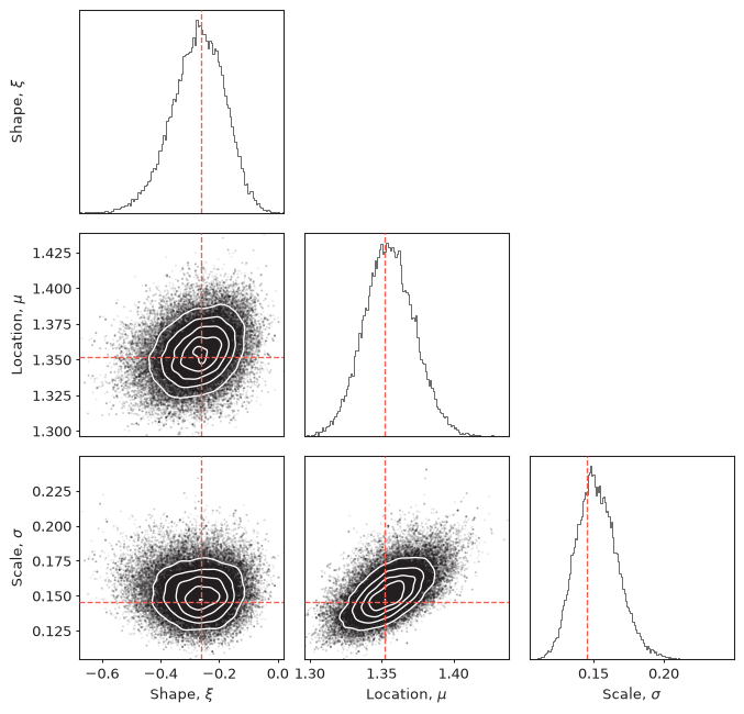
The posterior of the shape parameter lies almost entirely below zero, which, given scipy's sign convention for genextreme (see Distributions), indicates a heavy upper tail. The levels argument of plot_corner adds the given number of Gaussian KDE contours (white lines) to the off-diagonal plots. By default no contours are drawn.

Credible Intervals¶

Confidence intervals for MCMC (strictly speaking, Bayesian credible intervals) are calculated by computing return values for every posterior sample remaining after burn-in, and then taking quantiles of these return values. No additional fitting or resampling is required, so the n_samples argument used by MLE doesn't apply here:

summary = model.get_summary(
    return_period=[2, 5, 10, 25, 50, 100, 250, 500, 1000],
    alpha=0.95,
    burn_in=200,
)
print(summary)

               return value  lower ci  upper ci
return period
2.0                1.407873  1.373419  1.457470
5.0                1.619318  1.562467  1.735892
10.0               1.798414  1.706857  2.018379
25.0               2.081787  1.908044  2.553143
50.0               2.342852  2.072546  3.136436
100.0              2.654589  2.249358  3.944280
250.0              3.163149  2.500727  5.472215
500.0              3.637691  2.710593  7.158958
1000.0             4.207112  2.935657  9.475893

import numpy as np

model.plot_return_values(
    return_period=np.logspace(0.01, 3, 100),
    return_period_size="365.2425D",
    alpha=0.95,
    burn_in=200,
)

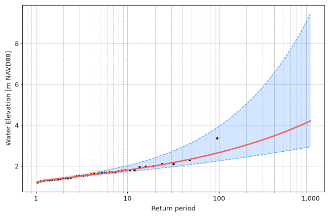
The return values are very close to those obtained using MLE, while the intervals for long return periods are shifted upwards and are wider (e.g. 2.25 to 3.94 m vs. 2.17 to 3.46 m for the 100-year water level). Uncertainty of rare events is dominated by uncertainty of the shape parameter, which the two methods capture differently - this is why it is useful to compare them.