Confidence Intervals
A return value on its own is only an estimate. Extreme value analysis extrapolates
from a limited number of observations to very rare events, so the uncertainty of
this estimate is often as important as the estimate itself
(see the warning in Extreme Value Types).
pyextremes quantifies this uncertainty using confidence intervals.
Getting Confidence Intervals
Confidence intervals are calculated when the alpha argument
(confidence interval width in the range (0, 1)) is passed to
get_return_value, get_summary, plot_return_values, or plot_diagnostic:
For alpha=0.95 the bounds are the 2.5% and 97.5% quantiles of
the return value estimates, i.e. the interval contains 95% of them.
Note
You can get the data and model variables referenced in this section
by running the following code:
import pandas as pd
from pyextremes import EVA

data = pd.read_csv(
    "battery_wl.csv",
    index_col=0,
    parse_dates=True,
).squeeze()
data = (
    data
    .sort_index(ascending=True)
    .astype(float)
    .dropna()
    .loc[pd.to_datetime("1925"):]
)
data = (
    data
    - (data.index.array - pd.to_datetime("1992"))
    / pd.to_timedelta("365.2425D")
    * 2.87e-3
)

model = EVA(data=data)
model.get_extremes("BM", block_size="365.2425D")
model.fit_model()
"battery_wl.csv"
can be downloaded here.
How the estimates are obtained depends on the model:
| Model | Method | Argument |
|---|---|---|
MLE, MOM, Lmoments |
bootstrap: refit the model to resampled extremes | n_samples (default 100) |
Emcee |
posterior samples from the MCMC trace | burn_in (default 0) |
Comparing Models
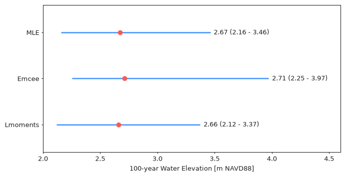
Different models estimate uncertainty in different ways, so it is worth comparing their confidence intervals. The figure below shows the 100-year water level and its 95% confidence interval for GEVD fitted to the annual maxima using three different models:
Code used to produce the figure above
import matplotlib.pyplot as plt
import numpy as np
from pyextremes import EVA
from pyextremes.plotting import pyextremes_rc

rows = []
for name, kwargs, ci_kwargs in [
    ("MLE", {}, {"n_samples": 1000}),
    ("Emcee", {"n_walkers": 100, "n_samples": 1000}, {"burn_in": 200}),
    ("Lmoments", {}, {"n_samples": 1000}),
]:
    model = EVA(data=data)
    model.get_extremes("BM", block_size="365.2425D")
    model.fit_model(model=name, distribution="genextreme", **kwargs)
    rows.append(
        (name, *model.get_return_value(return_period=100, alpha=0.95, **ci_kwargs))
    )

with plt.rc_context(rc=pyextremes_rc):
    fig, ax = plt.subplots(figsize=(8, 4), dpi=96)
    ax.grid(False)
    y = np.arange(len(rows))[::-1]
    for yi, (name, rv, lo, hi) in zip(y, rows):
        ax.plot([lo, hi], [yi, yi], color="#5199FF", lw=2, solid_capstyle="butt")
        ax.scatter([rv], [yi], s=40, color="#F85C50", zorder=10)
        ax.text(hi + 0.03, yi, f"{rv:.2f} ({lo:.2f} - {hi:.2f})", va="center")
    ax.set_yticks(y, [row[0] for row in rows])
    ax.set_ylim(-0.6, len(rows) - 0.4)
    ax.set_xlim(2.0, 4.6)
    ax.set_xlabel("100-year " + data.name)
All three models agree on the 100-year water level (~2.7 m), and their confidence
intervals mostly overlap. The intervals are strongly asymmetric: the upper bound is
much further from the estimate than the lower bound. This is typical for
heavy-tailed distributions, where a slightly larger shape parameter leads to a much
larger return value. The Emcee interval is the widest, because the posterior
captures the joint uncertainty of all parameters, including the shape parameter
(see Markov Chain Monte Carlo).
Number of Bootstrap Samples
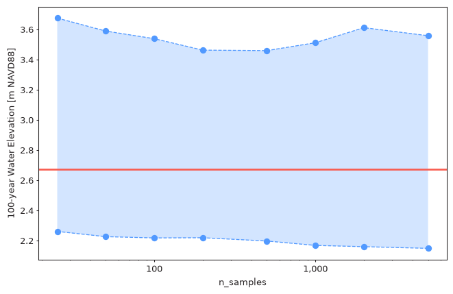
Bootstrap confidence intervals are estimated from a finite number of random
samples, so the bounds themselves are uncertain. The figure below shows how the
bounds of the 100-year water level change as n_samples increases:
n_samples |
Lower bound | Upper bound |
|---|---|---|
| 25 | 2.260 | 3.674 |
| 100 | 2.217 | 3.538 |
| 1000 | 2.167 | 3.511 |
| 5000 | 2.148 | 3.558 |
With few samples the bounds move noticeably every time more samples are added. After ~1000 samples the lower bound changes by less than 0.02 m, while the upper bound still varies by about ±0.05 m, because it depends on the few most extreme bootstrap samples. The default of 100 samples is suitable for exploring the data, but final results should use at least 1000 samples.
Tip
Bootstrap samples are cached on the model (see
Maximum Likelihood), so after calculating
intervals with n_samples=1000 once, subsequent calls with the same
or smaller n_samples are fast.
Interpreting Confidence Intervals
- Confidence intervals describe the uncertainty of the model (its parameters) given the data, assuming the model is correct. They don't account for the uncertainty of choosing the model itself, such as the distribution, block size, threshold, or declustering parameters. Use Threshold Selection and comparisons between distributions and models to assess that.
- Wide confidence intervals are a result in their own right: they indicate that the data doesn't contain enough information to estimate the return value reliably.
- Confidence intervals grow quickly with return period. Return values for return periods much longer than the observed record (e.g. a 1000-year value from 90 years of data) should be treated with caution, regardless of how narrow their confidence intervals are.