Diagnostic Plots

Before using return values, the fitted model should be checked visually. A model with a low AIC or a narrow confidence interval may still describe the data poorly, and plots are often the quickest way to notice that.

Diagnostic Plot¶

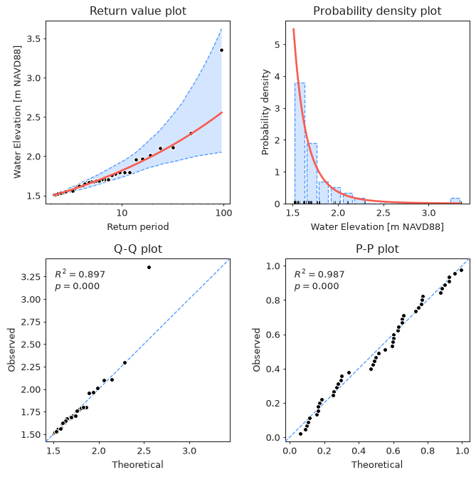
The plot_diagnostic method combines the four most commonly used plots in a single figure:

from pyextremes import EVA

model = EVA(data=data)
model.get_extremes("POT", threshold=1.5, r="24h")
model.fit_model()
model.plot_diagnostic(alpha=0.95)

import pandas as pd

data = pd.read_csv(
    "battery_wl.csv",
    index_col=0,
    parse_dates=True,
).squeeze()
data = (
    data
    .sort_index(ascending=True)
    .astype(float)
    .dropna()
    .loc[pd.to_datetime("1925"):]
)
data = (
    data
    - (data.index.array - pd.to_datetime("1992"))
    / pd.to_timedelta("365.2425D")
    * 2.87e-3
)

The plot_diagnostic method uses the following parameters:

• return_period - return periods for which the return value plot is drawn. If None (default), 100 return periods are spaced uniformly within the range of return periods of the observed extreme values.
• return_period_size - size of return period, by default 1 year.
• alpha - confidence interval width in the range (0, 1). If None (default), confidence intervals are not shown.
• plotting_position - plotting position used to assign empirical probabilities to the observed extreme values, by default "weibull". See Estimating Return Periods.
• figsize - figure size in inches in format (width, height), by default (8, 8).
• kwargs - model-specific arguments used to calculate confidence intervals: n_samples for MLE, MOM, and Lmoments models and burn_in for the Emcee model.

The method returns the figure and a tuple with the four axes (return values, PDF, Q-Q, and P-P), which can be used to customize the plot.

Components¶

Return Value Plot¶

The top left plot shows modeled return values (red line), their confidence interval (blue), and the observed extreme values (black dots) plotted at their empirical return periods. It is also available on its own via the plot_return_values method. A good model follows the observed values, especially for the largest ones. A systematic departure of the largest observed values from the curve indicates that the tail is not represented well.

Probability Density Plot¶

The top right plot shows a histogram of the extreme values, the probability density function of the fitted distribution (red line), and the individual extreme values (black ticks at the bottom). This plot shows whether the overall shape of the distribution is right, but it is not very informative about the tail, where there are only a few observations.

Q-Q Plot¶

The bottom left plot is a quantile-quantile (Q-Q) plot. Each observed extreme value (vertical axis) is plotted against the value which the fitted distribution predicts for the same empirical exceedance probability (horizontal axis). For a good model the points lie close to the dashed diagonal line. Because it is drawn in the units of the data, the Q-Q plot is the most sensitive of the four to problems in the tail.

The difference between a well-fitting and a poorly-fitting distribution is easy to see when comparing GEVD and Gumbel fitted to the annual maxima (see Distributions):

model.plot_probability(plot_type="QQ")

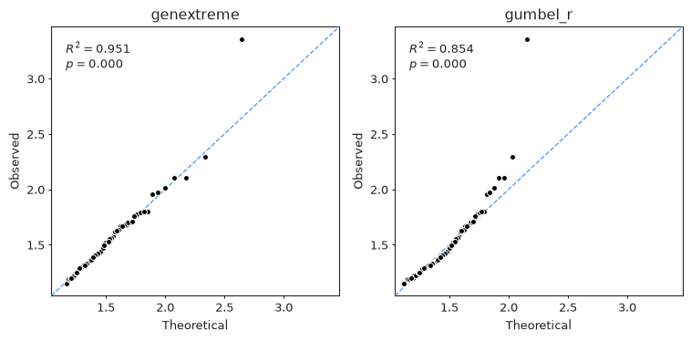
The Gumbel distribution can't represent the heavy upper tail of these data, so the largest observed values lie well above the diagonal. The largest value (Hurricane Sandy, 2012) is above the diagonal for both distributions, which is expected for the single most extreme event in ~90 years.

P-P Plot¶

The bottom right plot is a probability-probability (P-P) plot. It compares the empirical non-exceedance probability of each observed value (vertical axis) with the probability given by the fitted cumulative distribution function (horizontal axis):

model.plot_probability(plot_type="PP")

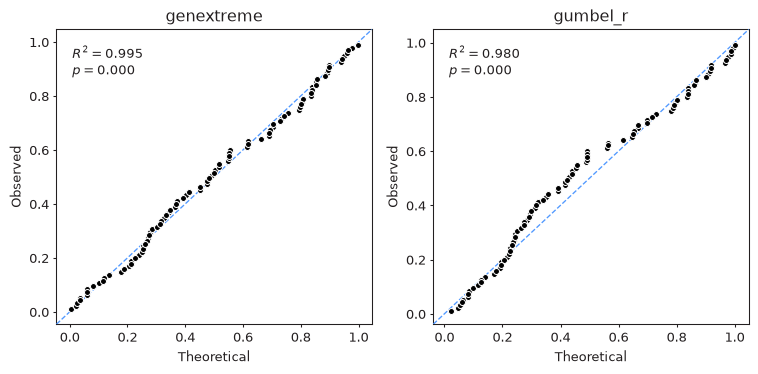
All probabilities are in the range [0, 1], so the P-P plot emphasizes the center of the distribution and is much less sensitive to the tail: Gumbel shows only a mild departure from the diagonal in the middle of the distribution, nothing like the clear misfit of the largest values visible in its Q-Q plot.

The plot_probability method uses the following parameters:

• plot_type - "QQ" for a Q-Q plot or "PP" for a P-P plot.
• return_period_size - size of return period, by default 1 year.
• plotting_position - plotting position, by default "weibull".
• ax - matplotlib Axes object. If provided, the plot is drawn on this axes. If None (default), a new figure and axes are created.
• figsize - figure size in inches in format (width, height), by default (8, 8).

import matplotlib.pyplot as plt
from pyextremes import EVA
from pyextremes.plotting import pyextremes_rc

models = {}
for distribution in ["genextreme", "gumbel_r"]:
    models[distribution] = EVA(data=data)
    models[distribution].get_extremes("BM", block_size="365.2425D")
    models[distribution].fit_model(distribution=distribution)

with plt.rc_context(rc=pyextremes_rc):
    fig, axes = plt.subplots(ncols=2, figsize=(8, 4), dpi=96)
    for ax, (distribution, model) in zip(axes, models.items()):
        model.plot_probability(plot_type="QQ", ax=ax)  # or "PP"
        ax.set_title(distribution)
    fig.tight_layout()

Other Plots¶

Other plots described elsewhere in this guide:

• extreme values extracted from the time series - plot_extremes, see Block Maxima and Peaks Over Threshold
• threshold selection plots, see Threshold Selection
• MCMC trace and corner plots - plot_trace and plot_corner, see Markov Chain Monte Carlo

All plotting methods of EVA are built on functions from the pyextremes.plotting module, which can be used directly with your own data (see the API Reference).