Maximum Likelihood
Maximum Likelihood Estimation (MLE) finds distribution parameters \(\theta\) which make the observed extreme values \(x_1, \dots, x_n\) most probable. This is done by maximizing the log-likelihood function:
where \(f\) is the probability density function of the distribution.
MLE is the default model in pyextremes and is the method used throughout
the classic EVA literature. It is fast, works with any continuous distribution,
and supports fixing any combination of distribution parameters.
Under the hood, pyextremes uses the fit method of
scipy.stats.rv_continuous.
Fitting the Model
Note
You can get the data variable referenced above by running the following code:
import pandas as pd

data = pd.read_csv(
    "battery_wl.csv",
    index_col=0,
    parse_dates=True,
).squeeze()
data = (
    data
    .sort_index(ascending=True)
    .astype(float)
    .dropna()
    .loc[pd.to_datetime("1925"):]
)
data = (
    data
    - (data.index.array - pd.to_datetime("1992"))
    / pd.to_timedelta("365.2425D")
    * 2.87e-3
)
"battery_wl.csv"
can be downloaded here.
The MLE model takes no additional arguments.
See Overview and Distributions
for the distribution and distribution_kwargs arguments.
Confidence Intervals
MLE produces a single best estimate of distribution parameters.
To estimate uncertainty of return values, pyextremes uses
bootstrap resampling:
- draw a random sample of the same size as the extreme values, with replacement, from the extreme values
- fit the distribution to this sample (keeping fixed parameters fixed)
- repeat
n_samplestimes and calculate return values for each set of fitted parameters - take quantiles of these return values as confidence interval bounds
(e.g. 2.5% and 97.5% for
alpha=0.95)
Confidence intervals are calculated when the alpha argument (confidence interval
width) is passed to get_summary, get_return_value, plot_return_values,
or plot_diagnostic. The number of bootstrap samples is controlled using the
n_samples argument (by default 100):
summary = model.get_summary(
    return_period=[2, 5, 10, 25, 50, 100, 250, 500, 1000],
    alpha=0.95,
    n_samples=1000,
)
print(summary)
               return value  lower ci  upper ci
return period
2.0                1.409343  1.371733  1.453128
5.0                1.622565  1.551648  1.701924
10.0               1.803499  1.685524  1.949140
25.0               2.090267  1.870731  2.399169
50.0               2.354889  2.020307  2.854903
100.0              2.671313  2.167416  3.456198
250.0              3.188356  2.392412  4.615462
500.0              3.671580  2.569467  5.815670
1000.0             4.252220  2.759888  7.544389
model = EVA(data=data)
model.get_extremes("POT", threshold=1.5, r="24h")
model.fit_model()
summary = model.get_summary(
    return_period=[5, 10, 25, 50, 100, 250, 500, 1000],
    alpha=0.95,
    n_samples=1000,
)
print(summary)
               return value  lower ci  upper ci
return period
5.0                1.660715  1.612644  1.736490
10.0               1.817443  1.718713  1.953821
25.0               2.069458  1.855135  2.353410
50.0               2.300945  1.945796  2.817342
100.0              2.574771  2.024709  3.441693
250.0              3.015076  2.096636  4.794305
500.0              3.419515  2.142378  6.232265
1000.0             3.897927  2.188766  8.248706
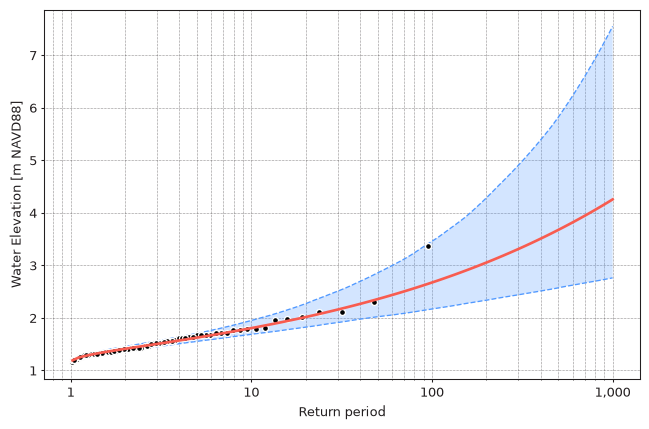
The same arguments are used to plot return values with confidence intervals:
import numpy as np

model.plot_return_values(
    return_period=np.logspace(0.01, 3, 100),
    return_period_size="365.2425D",
    alpha=0.95,
    n_samples=1000,
)
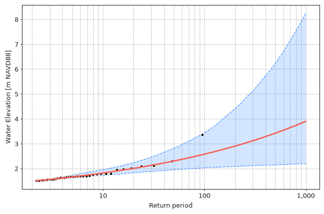
Return periods shorter than the extremes rate
Return values can only be calculated for return periods longer than the average
interval between extreme events. In the POT example above there are 44 extreme
values in ~93 years, so the shortest valid return period is ~2.1 years and a 2-year
return value is -inf. Block Maxima with 1-year blocks have exactly one extreme
value per year, so any return period longer than 1 year is valid.
Caching
Bootstrap samples are expensive to compute, so fitted parameters are cached
on the model and reused by subsequent calls. Requesting more samples
(e.g. n_samples=1000 after n_samples=100) only computes
the missing ones. Calculated return values are cached as well.
Both caches are discarded when the model is refitted.
Running as a script
When more than 50 new bootstrap samples are needed, they are calculated in
parallel using multiprocessing. When running pyextremes from a Python script
(as opposed to a Jupyter notebook), protect the entry point of your script with an
if __name__ == "__main__": block.
See Quick Start for more details.
Bootstrap confidence intervals depend on random samples, so they will be slightly
different every time they are calculated. Larger n_samples values produce more
stable confidence intervals at the cost of computation time.