Overview

Once extreme values are extracted, the next step is to fit a statistical model to them. Fitting a model means finding parameters of a continuous probability distribution (e.g. shape, location, and scale of the GEVD) which best describe the observed extreme values. The fitted distribution is then used to estimate return values for return periods well beyond the length of the observed record (e.g. a 100-year water level from 50 years of data).

In pyextremes a model is the method used to estimate distribution parameters (e.g. MLE or MCMC), while a distribution is the probability distribution whose parameters are estimated (e.g. GEVD or GPD). The two are chosen independently: any supported model can be used with any continuous distribution.

Available Models¶

MLE is the default model. It is fast, well understood, and is the method used throughout the classic EVA literature (e.g. Coles, 2001).

Fitting a Model¶

As outlined in the Read First section of this documentation, there are multiple ways the same thing can be achieved in pyextremes. A model can be fitted via:

• pyextremes.get_model - standalone function which takes a series of extreme values and returns a fitted model object
• pyextremes.EVA.fit_model - helper-class method (the model is not returned by this method, but instead is set on the EVA instance in the .model attribute)

The simplest way to fit a model is to use the default parameters:

from pyextremes import get_extremes, get_model

extremes = get_extremes(data, "BM", block_size="365.2425D")
model = get_model(
    model="MLE",
    extremes=extremes,
    distribution="genextreme",
)

from pyextremes import EVA

model = EVA(data=data)
model.get_extremes("BM", block_size="365.2425D")
model.fit_model()

import pandas as pd

data = pd.read_csv(
    "battery_wl.csv",
    index_col=0,
    parse_dates=True,
).squeeze()
data = (
    data
    .sort_index(ascending=True)
    .astype(float)
    .dropna()
    .loc[pd.to_datetime("1925"):]
)
data = (
    data
    - (data.index.array - pd.to_datetime("1992"))
    / pd.to_timedelta("365.2425D")
    * 2.87e-3
)

The EVA.fit_model method uses the following parameters:

• model - model name, one of "MLE" (default), "Emcee", "MOM", or "Lmoments".
• distribution - name of a distribution from scipy.stats (e.g. "genextreme") or a scipy.stats.rv_continuous object. By default the distribution is selected automatically based on the extreme value extraction method. See Distributions.
• distribution_kwargs - dictionary with distribution parameters to be held fixed, e.g. {"fc": 0} or {"floc": 1.5}. By default the location parameter is fixed for the GPD and Exponential distributions. See Distributions.
• kwargs - additional keyword arguments passed to the model. Only the Emcee model accepts additional arguments: n_walkers, n_samples, progress, and pool. See Markov Chain Monte Carlo.

The standalone get_model function takes the same arguments, except that it requires extremes and an explicit distribution, and doesn't fix any parameters unless distribution_kwargs is provided.

Inspecting the Model¶

Printing an EVA instance shows a summary of the data, extreme values, and the fitted model:

print(model)

                           Univariate Extreme Value Analysis
========================================================================================
                                      Source Data
----------------------------------------------------------------------------------------
Data label:    Water Elevation [m NAVD88]      Size:                             796,751
Start:                      November 1926      End:                           March 2020
========================================================================================
                                     Extreme Values
----------------------------------------------------------------------------------------
Count:                                 94      Extraction method:                     BM
Type:                                high      Block size:             365 days 05:49:12
========================================================================================
                                         Model
----------------------------------------------------------------------------------------
Model:                                MLE      Distribution:                  genextreme
Log-likelihood:                    18.026      AIC:                              -29.786
----------------------------------------------------------------------------------------
Free parameters:                 c=-0.266      Fixed parameters: All parameters are free
                                loc=1.353
                              scale=0.146
========================================================================================

The fitted model and its properties are available as attributes:

When using the standalone get_model function, the same attributes (distribution, fit_parameters, loglikelihood, and AIC) are available directly on the returned model object.

print(model.model.fit_parameters)

{'c': np.float64(-0.2657081538950403), 'loc': np.float64(1.3530417941848183), 'scale': np.float64(0.14625409987106597)}

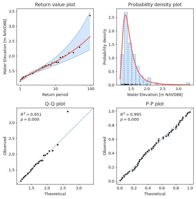
The quickest way to visually assess the fitted model is the diagnostic plot, which shows the return value plot, the probability density histogram, and the Q-Q and P-P plots (described in more detail in later sections):

model.plot_diagnostic(alpha=0.95)