Distributions

Extreme value theory tells us which distributions extreme values follow asymptotically, as the block size or threshold grows:

• Block Maxima follow the Generalized Extreme Value Distribution (GEVD), per the Fisher–Tippett–Gnedenko theorem
• Peaks Over Threshold follow the Generalized Pareto Distribution (GPD), per the Pickands–Balkema–De Haan theorem

Both distributions have a shape parameter which controls the behavior of the tail (i.e. how quickly return values grow with return period). When the shape parameter is zero, the GEVD reduces to the Gumbel distribution and the GPD reduces to the Exponential distribution. These are called degenerate cases: they have one parameter fewer and therefore produce narrower confidence intervals, but they cannot represent heavy (or bounded) tails.

pyextremes uses distributions from scipy.stats, which are referred to by name:

Default Distribution¶

When the distribution argument of EVA.fit_model is not provided, pyextremes fits two candidate distributions using the MLE model and selects the one with the smallest Akaike Information Criterion (AIC):

• genextreme or gumbel_r for extremes extracted using Block Maxima
• genpareto or expon for extremes extracted using Peaks Over Threshold (location parameter fixed at the threshold, see below)

The selected distribution is then fitted using the requested model. The AIC used by pyextremes is corrected for small sample sizes (AICc):

where \(k\) is the number of free distribution parameters, \(\hat{L}\) is the maximized likelihood, and \(n\) is the number of extreme values. AIC rewards goodness of fit and penalizes the number of parameters, so the degenerate distribution is selected unless the extra shape parameter improves the fit enough to justify it.

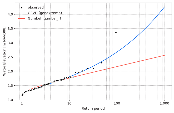
For the annual maxima of the Battery water levels, GEVD is clearly preferred:

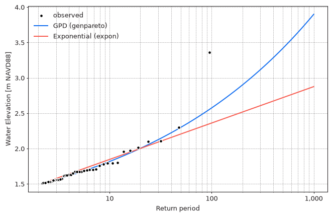
For the POT extremes above a threshold of 1.5 m (r="24h", see Threshold Selection) the difference is much smaller, but GPD is still preferred:

import matplotlib.pyplot as plt
import numpy as np
from pyextremes import EVA, get_return_periods
from pyextremes.plotting import pyextremes_rc

models = {}
for label, distribution in [
    ("GEVD (genextreme)", "genextreme"),
    ("Gumbel (gumbel_r)", "gumbel_r"),
]:
    models[label] = EVA(data)
    models[label].get_extremes("BM", block_size="365.2425D")
    models[label].fit_model(distribution=distribution)
    print(distribution, models[label].AIC)

observed = get_return_periods(
    ts=data,
    extremes=models["GEVD (genextreme)"].extremes,
    extremes_method="BM",
    extremes_type="high",
    block_size="365.2425D",
)
return_period = np.logspace(0.01, 3, 100)

with plt.rc_context(rc=pyextremes_rc):
    fig, ax = plt.subplots(figsize=(8, 5), dpi=96)
    ax.semilogx()
    ax.grid(True, which="both")
    ax.xaxis.set_major_formatter(plt.FuncFormatter(lambda x, _: f"{x:,.0f}"))
    ax.scatter(
        observed["return period"],
        observed.iloc[:, 0],
        s=20,
        lw=1,
        facecolor="k",
        edgecolor="w",
        zorder=20,
        label="observed",
    )
    for label, model in models.items():
        return_value, _, _ = model.get_return_value(return_period)
        ax.plot(return_period, return_value, lw=1.5, label=label)
    ax.set_xlabel("Return period")
    ax.set_ylabel(data.name)
    ax.legend(loc="upper left")

Selecting a Distribution¶

A distribution can be selected explicitly using the distribution argument:

from pyextremes import get_extremes, get_model

extremes = get_extremes(data, "BM", block_size="365.2425D")
model = get_model(
    model="MLE",
    extremes=extremes,
    distribution="gumbel_r",
)

from pyextremes import EVA

model = EVA(data=data)
model.get_extremes("BM", block_size="365.2425D")
model.fit_model(distribution="gumbel_r")

Any continuous distribution from scipy.stats can be used, either by name or by passing the distribution object (e.g. scipy.stats.genextreme). Custom distributions can be provided by subclassing scipy.stats.rv_continuous and passing an instance of the subclass.

Fixing Parameters¶

Any distribution parameter can be fixed (frozen) to a given value, in which case only the remaining (free) parameters are fitted. Fixed parameters are passed via the distribution_kwargs argument with names prefixed with f:

• fc - shape parameter(s), named after the parameter (c for genextreme and genpareto)
• floc - location parameter
• fscale - scale parameter

One use of this feature is to investigate degenerate models. For example, GEVD with a shape parameter fixed at 0 is the Gumbel distribution:

model.fit_model(
    distribution="genextreme",
    distribution_kwargs={"fc": 0},
)
print(model.model)

               MLE model
---------------------------------------
free parameters: loc=1.376, scale=0.171
fixed parameters: fc=0.000
AIC: -17.695
loglikelihood: 10.913
return value cache size: 0
fit parameter cache size: 0
---------------------------------------

The fitted location and scale parameters, log-likelihood, and AIC are identical to those of gumbel_r.

Location Parameter in POT¶

Exceedances over a threshold can't be smaller than the threshold itself, so the location parameter of the GPD and Exponential distributions is equal to the threshold by definition. Because of this, when a genpareto or expon distribution is fitted using EVA and distribution_kwargs is not provided, the location parameter is fixed:

• at the threshold for extremes extracted using Peaks Over Threshold
• at the smallest extreme value for extremes extracted using Block Maxima

This leaves only the shape and scale parameters to be fitted:

model = EVA(data=data)
model.get_extremes("POT", threshold=1.5, r="24h")
model.fit_model(distribution="genpareto")
print(model.model)

              MLE model
-------------------------------------
free parameters: c=0.242, scale=0.169
fixed parameters: floc=1.500
AIC: -42.985
loglikelihood: 23.639
return value cache size: 0
fit parameter cache size: 0
-------------------------------------

model = EVA(data=data)
model.get_extremes("POT", threshold=1.5, r="24h")
model.fit_model(distribution="genpareto", distribution_kwargs={})
print(model.model)

                   MLE model
------------------------------------------------
free parameters: c=0.255, loc=1.511, scale=0.153
fixed parameters: all parameters are free
AIC: -46.673
loglikelihood: 26.636
return value cache size: 0
fit parameter cache size: 0
------------------------------------------------

To fit all parameters freely, pass an empty dictionary (distribution_kwargs={}). Providing any distribution_kwargs replaces the default, so {"fc": 0} for genpareto would leave the location parameter free.